Machine Learning and Kernels

A common application of machine learning (ML) is the learning and classification of a set of raw data features by a ML algorithm or technique. In this context a ML kernel acts to the ML algorithm like sunshades, a telescope or a magnifying glass to the observing eye of a student learner. A good kernel filters the raw data and presents its features to the machine in a way that makes the learning task as simple as possible.

Historically a lot of progress in machine learning has been made in the development sophisticated learning algorithms, however selecting appropriate kernels remains a largely manual and time consuming task.

This post is inspired by a presentation by Prof. Mehryar Mohri about learning kernels. It reflects on the importance of kernels in support vector machines (SVM).

A total of three examples are presented. A linear kernel is shown to solve the first example but fails for the second task. There a square kernel is successful. Then a third example is presented for that both linear and square kernels are not sufficient. There a successful kernel can be generated out of a mixture of both base kernels. This illustrates that kernels can be generated out of bases, resulting in products that are more powerful in solving the task at hand than each individual components.

Support Vector Machines

Consider a support vector machine (SVM) for a classification task. Given a set of pairs of feature data-point vectors x and classifier labels y={-1,1}, the task of the SVM algorithm is to learn to group features x by classifiers. After training on a known data set the SVM machine is intended to correctly predict the class y of an previously unseen feature vector x.

Applications in quantitative finance of support vector machines include for example predictive tasks, where x consists of features derived from a historical stock indicator time series and y is a sell or buy signal. Another example could be that x consist of counts of key-words within a text such as an news announcements and y categorizes it again according on its impact to market movements. Outside of finance a text based SVM could be used to filter e-mail to be forwarded to either the inbox or the spam folder.

Linear Kernel

As indicated above the SVM works by grouping feature points according to its classifiers.
For illustration in the toy example below two dimensional feature vectors x={x1,x2} are generated in such a way that the class y=-1 points (triangles) are nicely separated from the class y=1 (circles).

The SVM algorithm finds the largest possible linear margin that separates these two regions. The marginal separators rest on the outpost points that are right on the front line of their respective regions. These points, marked as two bold triangles and one bold circle in the picture below, are named the ‘support vectors’ as they are supporting the separation boundary lines. In fact the SVM learning task fully consists of determining these support vector points and the margin distance that separates the regions. After training all other non-support points are not used for prediction.

In linear feature space the support vectors add to an overall hypothesis vector h, $h = \sum c_i x_i$ , such that the classification frontiers are given by the lines $h x + b = 1$ and $h x + b = -1$ centered around $h x + b = 0$ .

The code below utilizes the ksvm implementation in the R package ‘kernlab’, making use of “Jean-Philippe Vert’s” tutorials for graphing the classification separation lines.

require('kernlab')

kfunction <- function(linear =0, quadratic=0)
{
  k <- function (x,y)
 {
     linear*sum((x)*(y)) + quadratic*sum((x^2)*(y^2))
  }
  class(k) <- "kernel"
  k
}

n = 25
a1 = rnorm(n)
a2 = 1 - a1 + 2* runif(n)
b1 = rnorm(n)
b2 = -1 - b1 - 2*runif(n)
x = rbind(matrix(cbind(a1,a2),,2),matrix(cbind(b1,b2),,2))
y <- matrix(c(rep(1,n),rep(-1,n)))
                      
svp <- ksvm(x,y,type="C-svc",C = 100, kernel=kfunction(1,0),scaled=c())
plot(c(min(x[,1]), max(x[,1])),c(min(x[,2]), max(x[,2])),type='n',xlab='x1',ylab='x2')
title(main='Linear Separable Features')
ymat <- ymatrix(svp)
points(x[-SVindex(svp),1], x[-SVindex(svp),2], pch = ifelse(ymat[-SVindex(svp)] < 0, 2, 1))
points(x[SVindex(svp),1], x[SVindex(svp),2], pch = ifelse(ymat[SVindex(svp)] < 0, 17, 16))
   
# Extract w and b from the model   
w <- colSums(coef(svp)[[1]] * x[SVindex(svp),])
b <- b(svp)
   
# Draw the lines
abline(b/w[2],-w[1]/w[2])
abline((b+1)/w[2],-w[1]/w[2],lty=2)
abline((b-1)/w[2],-w[1]/w[2],lty=2)

Quadratic Kernel

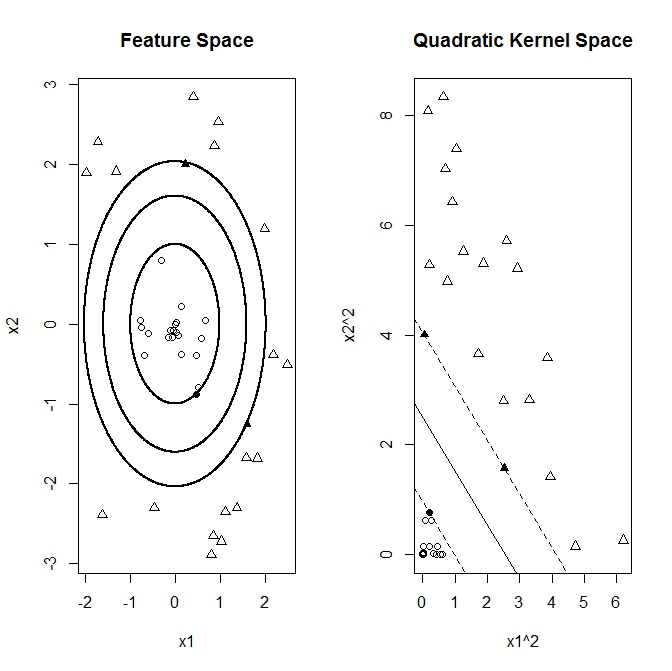
The following example illustrates a case where the feature points are non-linear separated. Points of the class y=1 (circles below) are placed in a inner region surrounded from all sides by points of class y=-1, again depicted as triangles. In this example there is no single straight (linear) line that can separate both regions. However here it is still possible to find such a separator by transforming the points $x=\{x_1, x_2\}$ from feature space to a quadratic kernel space with points given by the corresponding square coordinates $\{x_1^2, x_2^2\}$ .

The technique of transforming from feature space into a measure that allows for a linear separation can be formalized in terms of kernels. Assuming $\Phi()$ is a vector coordinate transformation function. For example a squared coordinate space would be $\{ \Phi(x)_1 , \Phi(x)_2 \} = \{ x_1^2 , x_2^2 \}$ . The SVM separation task is now acting on in the transformed space to find the support vectors that generate

$h \Phi(x) + b = \pm 1$

for the hypothesis vector $h = \sum c_i \Phi(x_i)$ given by the sum over support vector points $x_i$ . Putting both expressions together we get

$\sum c_i K(x_i,x) + b = \pm 1$

with the scalar kernel function $K(x_i,x) = \Phi(x_i) \Phi(x)$ . The kernel is composed out of the scalar product between a support vector $x_i$ and another feature vector point $x$ in the transformed space.

In practice the SVM algorithm can be fully expressed in terms of kernels without having to actually specify the feature space transformation. Popular kernels are for example higher powers of the linear scalar product (polynomial kernel). Another example is a probability weighed distance between two points (Gaussian kernel).

Implementing a two dimensional quadratic kernel function allows the SVM algorithm to find support vectors and correctly separate the regions. Below the graph below illustrates that the non-linear regions are linearly separated after transforming to the squared kernel space.

The “R” implementation makes use of ksvm’s flexibility to allow for custom kernel functions. The function ‘kfunction’ returns a linear scalar product kernel for parameters (1,0) and a quadratic kernel function for parameters (0,1).

require('kernlab')
kfunction <- function(linear =0, quadratic=0)
{
  k <- function (x,y)
 {
     linear*sum((x)*(y)) + quadratic*sum((x^2)*(y^2))
  }
  class(k) <- "kernel"
  k
}

n = 20
r = runif(n)
a = 2*pi*runif(n)
a1 = r*sin(a)
a2 = r*cos(a)
r = 2+runif(n)
a = 2*pi*runif(n)
b1 = r*sin(a)
b2 = r*cos(a)
x = rbind(matrix(cbind(a1,a2),,2),matrix(cbind(b1,b2),,2))
y <- matrix(c(rep(1,n),rep(-1,n)))
                          
svp <- ksvm(x,y,type="C-svc",C = 100, kernel=kfunction(0,1),scaled=c())
par(mfrow=c(1,2))
plot(c(min(x[,1]), max(x[,1])),c(min(x[,2]), max(x[,2])),type='n',xlab='x1',ylab='x2')
title(main='Feature Space')
ymat <- ymatrix(svp)
points(x[-SVindex(svp),1], x[-SVindex(svp),2], pch = ifelse(ymat[-SVindex(svp)] < 0, 2, 1))
points(x[SVindex(svp),1], x[SVindex(svp),2], pch = ifelse(ymat[SVindex(svp)] < 0, 17, 16))
   
# Extract w and b from the model   
w2 <- colSums(coef(svp)[[1]] * x[SVindex(svp),]^2)
b <- b(svp)

x1 = seq(min(x[,1]),max(x[,1]),0.01)
x2 = seq(min(x[,2]),max(x[,2]),0.01)

points(-sqrt((b-w2[1]*x2^2)/w2[2]), x2, pch = 16 , cex = .1 )
points(sqrt((b-w2[1]*x2^2)/w2[2]), x2, pch = 16 , cex = .1 )
points(x1, sqrt((b-w2[2]*x1^2)/w2[1]), pch = 16 , cex = .1 )
points(x1,  -sqrt((b-w2[2]*x1^2)/w2[1]), pch = 16, cex = .1 )

points(-sqrt((1+ b-w2[1]*x2^2)/w2[2]) , x2, pch = 16 , cex = .1 )
points( sqrt((1 + b-w2[1]*x2^2)/w2[2]) , x2,  pch = 16 , cex = .1 )
points( x1 , sqrt(( 1 + b -w2[2]*x1^2)/w2[1]), pch = 16 , cex = .1 )
points( x1 , -sqrt(( 1 + b -w2[2]*x1^2)/w2[1]), pch = 16, cex = .1 )

points(-sqrt((-1+ b-w2[1]*x2^2)/w2[2]) , x2, pch = 16 , cex = .1 )
points( sqrt((-1 + b-w2[1]*x2^2)/w2[2]) , x2,  pch = 16 , cex = .1 )
points( x1 , sqrt(( -1 + b -w2[2]*x1^2)/w2[1]), pch = 16 , cex = .1 )
points( x1 , -sqrt(( -1 + b -w2[2]*x1^2)/w2[1]), pch = 16, cex = .1 )

xsq <- x^2
svp <- ksvm(xsq,y,type="C-svc",C = 100, kernel=kfunction(1,0),scaled=c())

plot(c(min(xsq[,1]), max(xsq[,1])),c(min(xsq[,2]), max(xsq[,2])),type='n',xlab='x1^2',ylab='x2^2')
title(main='Quadratic Kernel Space')
ymat <- ymatrix(svp)
points(xsq[-SVindex(svp),1], xsq[-SVindex(svp),2], pch = ifelse(ymat[-SVindex(svp)] < 0, 2, 1))
points(xsq[SVindex(svp),1], xsq[SVindex(svp),2], pch = ifelse(ymat[SVindex(svp)] < 0, 17, 16))
   
# Extract w and b from the model   
w <- colSums(coef(svp)[[1]] * xsq[SVindex(svp),])
b <- b(svp)
   
# Draw the lines
abline(b/w[2],-w[1]/w[2])
abline((b+1)/w[2],-w[1]/w[2],lty=2)
abline((b-1)/w[2],-w[1]/w[2],lty=2)

Alignment and Kernel Mixture

The final exploratory feature data set consists again of two classes of points within two dimensional space. This time two distinct regions of points are separated by a parabolic boundary, where vector points of class y=1 (circles) are below and y=-1 (triangles) are above the separating curve. The example is selected for its property that neither the linear nor the quadratic kernels alone are able to resolve the SVM classification problem.

The second graph below illustrates that feature points of both classes are scattered onto overlapping regions in the quadratic kernel space. It indicates that for this case the sole utilization of the quadratic kernel is not enough to resolve the classification problem.

In “Algorithms for Learning Kernels Based on Centered Alignment” Corinna Cortes, Mehryar Mohri and Afshin Rostamizadeh compose mixed kernels out of base kernel functions. This is perhaps similar to how a vector can be composed out of its coordinate base vectors or a function can be assembled in functional Hilbert space.

In our example we form a new mixed kernel out of the linear and the quadratic kernels $K_1$ and $K_2$

$K_M(x,z) = \rho_1 K_1(x,z) + \rho_2 K_2(x,z)$

The graph below demonstrate that the mixed kernel successfully solves the classification problem even thought each individual base kernels are insufficient on its own. In experimentation the actual values of the mixture weights $\rho_1$ , $\rho_2$ are not critical. Following the study above we choose the weights according to how much each individual base kernel on its individual aligned with the raw classification matrix $Y = y^T y$ composed out of the classifier vector $y$ .

Alignment is based on the observation that a perfectly selected kernel matrix $K_{i,j} = K(x_i,x_j)$ would trivially solve the classification problem if its elements are equal to the $Y$ matrix. In that case choosing an arbitrary vector $x_1$ as support the the kernel $K(x_1, x_i)$ would give $1$ if $x_1$ and $x_i$ are in the same category and $-1$ otherwise.

Similar to the concept of correlation, kernel alignment between two kernels is defined by the expectation over the feature space, resulting in matrix products

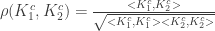
$\rho ( K^c_1 , K^c_2 ) = \frac{ < K^c_1 , K^c_2 > }{ \sqrt{ < K^c_1 , K^c_1 > < K^c_2 , K^c_2 > } }$

with the product $latex = Tr[A^T B]$. The expectation is take assuming centered $n \times n$ kernel matrices according to $K^c = (I-(11^T)/n)K(I-(11^T)/n)$ . (For details see reference above.)

Kernel matrix centering and alignment functions are implemented in the ‘R’ as following

require('kernlab')

n = 100
a1 = 4*runif(n)-2
a2 = 1 - a1^2 - 0.5 - 2*runif(n)
b1 = 4*runif(n)-2
b2 = 1 - b1^2 + 0.5 + 2*runif(n)

x = rbind(matrix(cbind(a1,a2),,2),matrix(cbind(b1,b2),,2))
y <- matrix(c(rep(1,n),rep(-1,n)))

kfunction <- function(linear, quadratic)
{
  k <- function (x,y)
 {
     linear*sum((x)*(y)) + quadratic*sum((x^2)*(y^2))
  }
  class(k) <- "kernel"
  k
}

center_kernel <- function(kernel)
{
m <- length(kernel[,1])
ones <- matrix(rep(1,m),m)
(diag(m) - ones %*% t(ones) / m)*kernel*(diag(m) - ones %*% t(ones) / m)
}
f_product<- function(x,y)
{
    sum(diag(crossprod(t(x),y)))
}
f_norm<- function(x)
{
    sqrt(f_product(x,x))
}
kernel_alignment <- function(x,y)
{
    f_product(x,y)/(f_norm(x)*f_norm(y))
}
                          
x_kernel1 <- kernelMatrix(kfunction(1,0),x)
y_kernel   <- y %*% t(y)
x_kernel2 <- kernelMatrix(kfunction(0,1),x)

x_kernel1_c <- center_kernel(x_kernel1)
x_kernel2_c <- center_kernel(x_kernel2)

y_kernel_c <- center_kernel(y_kernel)

alignment1 <- kernel_alignment(x_kernel1_c,y_kernel_c)
alignment2 <- kernel_alignment(x_kernel2_c,y_kernel_c)

x_kernel3 <- kernelMatrix(kfunction(alignment1, alignment2),x)
x_kernel3_c <- center_kernel(x_kernel3)
alignment3 <- kernel_alignment(x_kernel3_c,y_kernel_c)

svp <- ksvm(x,y,type="C-svc",C = 100, kernel=kfunction(alignment1,alignment2), scaled=c())
par(mfrow=c(2,1))
plot(c(min(x[]), max(x[])), c(min(x[]), max(x[])),type='n',xlab='x1',ylab='x2')
title(main='Parabolic Featureset (Mixed Kernel SVM)')
ymat <- ymatrix(svp)
points(x[-SVindex(svp),1], x[-SVindex(svp),2], pch = ifelse(ymat[-SVindex(svp)] < 0, 2, 1))
points(x[SVindex(svp),1], x[SVindex(svp),2], pch = ifelse(ymat[SVindex(svp)] < 0, 17, 16))
   
# Extract w and b from the model   
w <- colSums(coef(svp)[[1]] * (alignment1*x[SVindex(svp),]))
v <- colSums(coef(svp)[[1]] * (alignment2*x[SVindex(svp),]^2))
b <- b(svp)

x1 = seq(min(x[]),max(x[]),0.01)
x2 = seq(min(x[]),max(x[]),0.01)

points( sqrt( (b-w[2]*x2-v[2]*x2^2)/v[1] + (w[1]/(2*v[1]))^2 ) - w[1]/(2*v[1]) , x2, pch = 16, cex = .1 )
points( -sqrt( (b-w[2]*x2-v[2]*x2^2)/v[1] + (w[1]/(2*v[1]))^2 ) - w[1]/(2*v[1]) , x2, pch = 16, cex = .1 )
points( x1, sqrt( (b-w[1]*x1-v[1]*x1^2)/v[2] + (w[2]/(2*v[2]))^2 ) - w[2]/(2*v[2]) , pch = 16, cex = .1 )
points( x1, -sqrt( (b-w[1]*x1-v[1]*x1^2)/v[2] + (w[2]/(2*v[2]))^2 ) - w[2]/(2*v[2]) , pch = 16, cex = .1 )

points( sqrt( (1+ b-w[2]*x2-v[2]*x2^2)/v[1] + (w[1]/(2*v[1]))^2 ) - w[1]/(2*v[1]) , x2, pch = 16, cex = .1 )
points( -sqrt( (1 + b-w[2]*x2-v[2]*x2^2)/v[1] + (w[1]/(2*v[1]))^2 ) - w[1]/(2*v[1]) , x2, pch = 16, cex = .1 )
points( x1, sqrt( (1+b-w[1]*x1-v[1]*x1^2)/v[2] + (w[2]/(2*v[2]))^2 ) - w[2]/(2*v[2]) , pch = 16, cex = .1 )
points( x1, -sqrt( (1+b-w[1]*x1-v[1]*x1^2)/v[2] + (w[2]/(2*v[2]))^2 ) - w[2]/(2*v[2]) , pch = 16, cex = .1 )

points( sqrt( (-1+ b-w[2]*x2-v[2]*x2^2)/v[1] + (w[1]/(2*v[1]))^2 ) - w[1]/(2*v[1]) , x2, pch = 16, cex = .1 )
points( -sqrt( (-1 + b-w[2]*x2-v[2]*x2^2)/v[1] + (w[1]/(2*v[1]))^2 ) - w[1]/(2*v[1]) , x2, pch = 16, cex = .1 )
points( x1, sqrt( (-1+b-w[1]*x1-v[1]*x1^2)/v[2] + (w[2]/(2*v[2]))^2 ) - w[2]/(2*v[2]) , pch = 16, cex = .1 )
points( x1, -sqrt( (-1+b-w[1]*x1-v[1]*x1^2)/v[2] + (w[2]/(2*v[2]))^2 ) - w[2]/(2*v[2]) , pch = 16, cex = .1 )

plot(x[]^2,type='n',xlab='x1^2',ylab='x2^2')
title(main='Not Linear Separable in Quadratic Kernel Coordinates')
points(x[1:100,]^2,pch=16)
points(x[101:200,]^2,pch=2)

In conclusion this post attempts to illuminate the importance role of kernel selection in machine learning and demonstrates the use of kernel mixture techniques. Kernel weights were chosen somewhat ad-hoc by alignments to the target classifiers, thus preceding the actual SVM learning phase. More sophisticated algorithms and techniques that automate and combine these steps are a topic of current ongoing research.

3 Responses to Learning Kernels SVM

Jonathan Shore says:

September 27, 2012 at 12:02 am

very nice post illustrating the power of kernels!

Pingback: NIPS Data Science Review Part 1 : Engineering Rich Relevance Blog
Alex Diana says:

April 24, 2016 at 9:57 pm

There is an error in the Quadratic Kernel code. The lines 39-52 have got w[1] and w[2] flipped. In this example, it doesn’t make any difference, but in general it does.

Learning Kernels SVM

Machine Learning and Kernels

Support Vector Machines

Linear Kernel

Quadratic Kernel

Alignment and Kernel Mixture

3 Responses to Learning Kernels SVM

Leave a comment Cancel reply

Blogroll

Community

Education

Resource

Learning Kernels SVM

Machine Learning and Kernels

Support Vector Machines

Linear Kernel

Quadratic Kernel

Alignment and Kernel Mixture

Share this:

Related

3 Responses to Learning Kernels SVM

Leave a comment Cancel reply

Blogroll

Community

Education

Resource